Crime is an international concern, but it is documented and handled in very different ways in different countries. In the United States, violent crimes and property crimes are recorded by the Federal Bureau of Investigation (FBI). Additionally, each city documents crime, and some cities release data regarding crime rates. The city of Chicago, Illinois releases crime data from 2001 onward online.

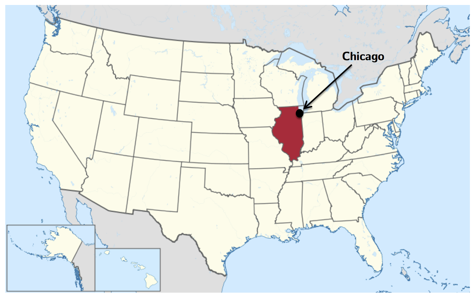
Chicago is the third most populous city in the United States, with a population of over 2.7 million people. The city of Chicago is shown in the map below, with the state of Illinois highlighted in red.

There are two main types of crimes: violent crimes, and property crimes. In this problem, we'll focus on one specific type of property crime, called "motor vehicle theft" (sometimes referred to as grand theft auto). This is the act of stealing, or attempting to steal, a car. In this problem, we'll use some basic data analysis in R to understand the motor vehicle thefts in Chicago.

Please download the file mvtWeek1.csv for this problem (do not open this file in any spreadsheet software before completing this problem because it might change the format of the Date field).

mvt = read.csv("mvtWeek1.csv")
str(mvt)

• Date: the date the crime occurred
• LocationDescription: the location where the crime occurred
• Arrest: whether or not an arrest was made for the crime (TRUE if an arrest was made, and FALSE if an arrest was not made)
• Domestic: whether or not the crime was a domestic crime, meaning that it was committed against a family member (TRUE if it was domestic, and FALSE if it was not domestic)
• Beat: the area, or "beat" in which the crime occurred. This is the smallest regional division defined by the Chicago police department.
• District: the police district in which the crime occured. Each district is composed of many beats, and are defined by the Chicago Police Department.
• CommunityArea: the community area in which the crime occurred. Since the 1920s, Chicago has been divided into what are called "community areas", of which there are now 77. The community areas were devised in an attempt to create socially homogeneous regions.
• Year: the year in which the crime occurred.
• Latitude: the latitude of the location at which the crime occurred.
• Longitude: the longitude of the location at which the crime occurred.

Dataset contains 191641 obs. of 11 variables. 9181151 is the maximum value of the variable "ID".

max(mvt$ID)

If we type summary(mvt) in your R console, we can see the summary statistics for each variable. This shows that the minimum value of Beat is 111. Alternatively, we could use the min function by typing min(mvt$Beat).

summary(mvt)
min(mvt$Beat)

If we type summary(mvt) in your R console, we can see the summary statistics for each variable. This shows that 15,536 observations fall under the category TRUE for the variable Arrest.

summary(mvt)

This also shows that 2,308 observations fall under the category ALLEY for the variable LocationDescription. We can also read this from:

table(mvt$LocationDescription)

Understanding Dates in R

In many datasets, like this one, you have a date field. Unfortunately, R does not automatically recognize entries that look like dates. We need to use a function in R to extract the date and time. If we type

mvt$Date[1]

in our R console, we can see that the first entry is 12/31/12 23:15. It is in the format Month/Day/Year Hour:Minute. Now, let's convert these characters into a Date object in R. In your R console, type

DateConvert = as.Date(strptime(mvt$Date, "%m/%d/%y %H:%M"))

This converts the variable "Date" into a Date object in R. Now, let's extract the month and the day of the week, and add these variables to our data frame mvt. We can do this with two simple functions by typing the following commands in R:

mvt$Month = months(DateConvert)
mvt$Weekday = weekdays(DateConvert)

This creates two new variables in our data frame, Month and Weekday, and sets them equal to the month and weekday values that we can extract from the Date object. Lastly, replace the old Date variable with DateConvert by typing:

mvt$Date = DateConvert

If we type

table(mvt$Month)

we can see that the month with the smallest number of observations is February. If we type

table(mvt$Weekday)

we can see that the weekday with the largest number of observations is Friday. Each observation in the dataset represents a motor vehicle theft, and the Arrest variable indicates whether an arrest was later made for this theft. If we type

table(mvt$Arrest,mvt$Month)

we can see that the largest number of observations with Arrest=TRUE occurs in the month of January.

Now, let's make some plots to help us better understand how crime has changed over time in Chicago. Throughout this problem, and in general, you can save your plot to a file.

Visualizing Crime Trends

First, let's make a histogram of the variable Date. We'll add an extra argument, to specify the number of bars we want in our histogram. In our R console, type:

hist(mvt$Date, breaks=100)

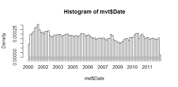
Looking at the histogram, it looks like crime generally decreases from 2002 - 2012. From 2005 - 2008, there is a clear downward trend in crime. From 2009 - 2011, there is a clear upward trend in crime.

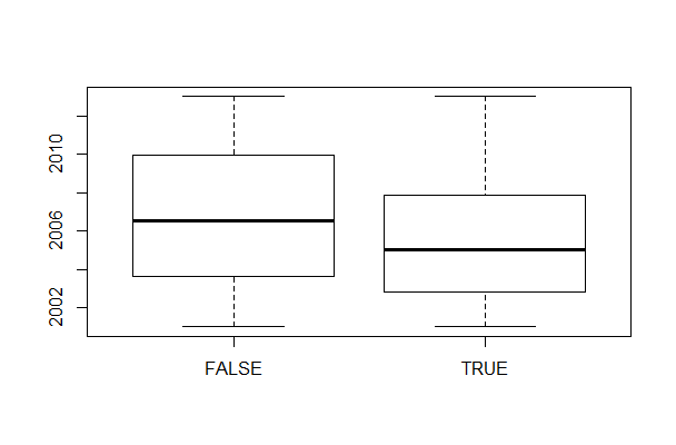
Now, let's see how arrests have changed over time. Create a boxplot of the variable "Date", sorted by the variable "Arrest". In a boxplot, the bold horizontal line is the median value of the data, the box shows the range of values between the first quartile and third quartile, and the whiskers (the dotted lines extending outside the box) show the minimum and maximum values, excluding any outliers (which are plotted as circles). Outliers are defined by first computing the difference between the first and third quartile values, or the height of the box. This number is called the Inter-Quartile Range (IQR). Any point that is greater than the third quartile plus the IQR or less than the first quartile minus the IQR is considered an outlier.

 boxplot(mvt$Date ~ mvt$Arrest)

If we look at the boxplot, the one for Arrest=TRUE is definitely skewed towards the bottom of the plot, meaning that there were more crimes for which arrests were made in the first half of the time period.

If we create a table using the command

table(mvt$Arrest, mvt$Year)

• The column for 2001 has 2152 observations with Arrest=TRUE and 18517 observations with Arrest=FALSE. The fraction of motor vehicle thefts in 2001 for which an arrest was made is thus 2152/(2152+18517) = 0.1041173.
• The column for 2007 has 1212 observations with Arrest=TRUE and 13068 observations with Arrest=FALSE. The fraction of motor vehicle thefts in 2007 for which an arrest was made is thus 1212/(1212+13068) = 0.08487395.
• The column for 2012 has 550 observations with Arrest=TRUE and 13542 observations with Arrest=FALSE. The fraction of motor vehicle thefts in 2012 for which an arrest was made is thus 550/(550+13542) = 0.03902924. Since there may still be open investigations for recent crimes, this could explain the trend we are seeing in the data. There could also be other factors at play, and this trend should be investigated further. However, since we don't know when the arrests were actually made, our detective work in this area has reached a dead end.

Popular Locations

Analyzing this data could be useful to the Chicago Police Department when deciding where to allocate resources. If they want to increase the number of arrests that are made for motor vehicle thefts, where should they focus their efforts?

Let's find the top five locations where motor vehicle thefts occur. If we create a table of the LocationDescription variable, it is unfortunately very hard to read since there are 78 different locations in the data set. By using the sort function, we can view this same table, but sorted by the number of observations in each category. In your R console, type:

sort(table(mvt$LocationDescription))

The locations with the largest number of motor vehicle thefts are Street, Parking Lot/Garage (Non. Resid.), Alley, Gas Station, and Driveway - Residential.

Let's create a subset of our data, only taking observations for which the theft happened in one of these five locations, and call this new data set "Top5". To do this, we can use the | symbol. This is also called a logical "or" operation. Alternately, we could create five different subsets, and then merge them together into one data frame using rbind.

Top5 = subset(mvt, LocationDescription=="STREET" | LocationDescription=="PARKING LOT/GARAGE(NON.RESID.)" | LocationDescription=="ALLEY" | LocationDescription=="GAS STATION" | LocationDescription=="DRIVEWAY - RESIDENTIAL")

If we look at the structure of this data frame with str(Top5), we can see that there are 177510 observations.

Another way of doing this would be to use the %in% operator in R. This operator checks for inclusion in a set. We can create the same subset by typing the following two lines in your R console:

TopLocations = c("STREET", "PARKING LOT/GARAGE(NON.RESID.)", "ALLEY", "GAS STATION", "DRIVEWAY - RESIDENTIAL")
Top5 = subset(mvt, LocationDescription %in% TopLocations)

R will remember the other categories of the LocationDescription variable from the original dataset, so running table(Top5$LocationDescription) will have a lot of unnecessary output. To make our tables a bit nicer to read, we can refresh this factor variable. In your R console, type:

Top5$LocationDescription = factor(Top5$LocationDescription)

If we run the str or table function on Top5 now, we should see that LocationDescription now only has 5 values, as we expect.

If we create a table of LocationDescription compared to Arrest,

table(Top5$LocationDescription, Top5$Arrest)

we can then compute the fraction of motor vehicle thefts that resulted in arrests at each location. Gas Station has by far the highest percentage of arrests, with over 20% of motor vehicle thefts resulting in an arrest.

On Saturday the most motor vehicle thefts at gas stations happen. This can be read from

table(Top5$LocationDescription, Top5$Weekday).

Also, Saturday is the day of the week with the fewest motor vehicle thefts in residential driveways.

table(Top5$LocationDescription, Top5$Weekday)