Flu epidemics constitute a major public health concern causing respiratory illnesses, hospitalizations, and deaths. According to the National Vital Statistics Reports published in October 2012, influenza ranked as the eighth leading cause of death in 2011 in the United States. Each year, 250,000 to 500,000 deaths are attributed to influenza related diseases throughout the world.

The U.S. Centers for Disease Control and Prevention (CDC) and the European Influenza Surveillance Scheme (EISS) detect influenza activity through virologic and clinical data, including Influenza-like Illness (ILI) physician visits. Reporting national and regional data, however, are published with a 1-2 week lag.

The Google Flu Trends project was initiated to see if faster reporting can be made possible by considering flu-related online search queries -- data that is available almost immediately.

We would like to estimate influenza-like illness (ILI) activity using Google web search logs. Fortunately, one can easily access this data online: ILI Data - The CDC publishes on its website the official regional and state-level percentage of patient visits to healthcare providers for ILI purposes on a weekly basis. Google Search Queries - Google Trends allows public retrieval of weekly counts for every query searched by users around the world. For each location, the counts are normalized by dividing the count for each query in a particular week by the total number of online search queries submitted in that location during the week. Then, the values are adjusted to be between 0 and 1.

The csv file FluTrain.csv aggregates this data from January 1, 2004 until December 31, 2011 as follows:

• "Week" - The range of dates represented by this observation, in year/month/day format.

• "ILI" - This column lists the percentage of ILI-related physician visits for the corresponding week.

• "Queries" - This column lists the fraction of queries that are ILI-related for the corresponding week, adjusted to be between 0 and 1 (higher values correspond to more ILI-related search queries).

Before applying analytics tools on the training set, we first need to understand the data at hand. Let's load "FluTrain.csv" into a data frame called FluTrain.

Looking at the time period 2004-2011, let's find out which week corresponds to the highest percentage of ILI-related physician visits. We can use which.max(FluTrain$ILI) to find the row number corresponding to the observation with the maximum value of ILI, which is 303. Then, we can output the corresponding week using

which.max(FluTrain$ILI)
FluTrain$Week[303]

Let us now understand the data at an aggregate level by plotting the histogram of the dependent variable, ILI.

hist(FluTrain$ILI)

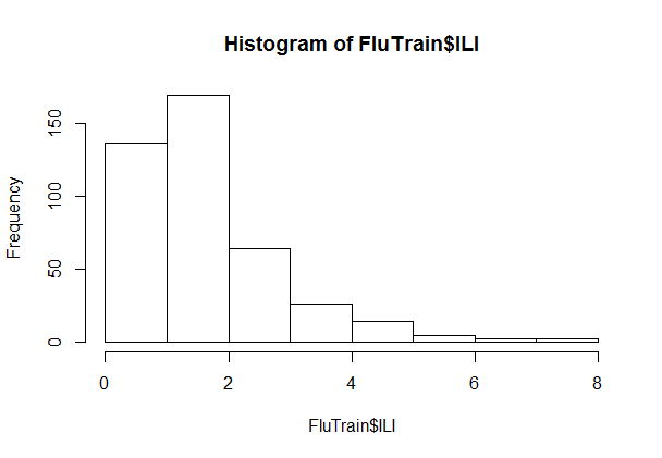
Most of the ILI values are small, with a relatively small number of much larger values (in statistics, this sort of data is called "skew right").

When handling a skewed dependent variable, it is often useful to predict the logarithm of the dependent variable instead of the dependent variable itself -- this prevents the small number of unusually large or small observations from having an undue influence on the sum of squared errors of predictive models. In this problem, we will predict the natural log of the ILI variable, which can be computed in R using the log() function.

The plot can be obtained with:

plot(FluTrain$Queries, log(FluTrain$ILI))

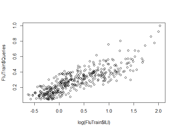
Visually, there is a positive, linear relationship between log(ILI) and Queries.

Based on the plot we just made, it seems that a linear regression model could be a good modeling choice. Based on our understanding of the data from the previous subproblem, this model best describes our estimation problem:

log(ILI) = intercept + coefficient x Queries, where the coefficient is positive

The model can be trained with:

FluTrend1 = lm(log(ILI)~Queries, data=FluTrain)

From summary(FluTrend1), we read that the R-squared value is 0.709.

For a single variable linear regression model, there is a direct relationship between the R-squared and the correlation between the independent and the dependent variables.

Correlation = cor(FluTrain$Queries, log(FluTrain$ILI))

The values of the three expressions are then:

Correlation^2 = 0.7090201

It appears that Correlation^2 is equal to the R-squared value.

The csv file FluTest.csv provides the 2012 weekly data of the ILI-related search queries and the observed weekly percentage of ILI-related physician visits. Load this data into a data frame called FluTest.

Normally, we would obtain test-set predictions from the model FluTrend1 using the code

PredTest1 = predict(FluTrend1, newdata=FluTest)

However, the dependent variable in our model is log(ILI), so PredTest1 would contain predictions of the log(ILI) value. We are instead interested in obtaining predictions of the ILI value. We can convert from predictions of log(ILI) to predictions of ILI via exponentiation, or the exp() function. The new code, which predicts the ILI value, is

PredTest1 = exp(predict(FluTrend1, newdata=FluTest))

For example in order to get the estimate for the percentage of ILI-related physician visits for the week of March 11, 2012, we need to type in our R console:

PredTest1[which(FluTest$Week == "2012-03-11 - 2012-03-17")]

The predicted value is 2.187383.

The actual value is the 11th testing set ILI value or FluTest$ILI[11], which has value 2.293422. Finally we can compute the relative error to be (2.293422 - 2.187378)/2.293422 = 0.04624

The RMSE can be calculated by first computing the SSE:

SSE = sum((PredTest1-FluTest$ILI)^2)

RMSE = sqrt(SSE / nrow(FluTest))

Alternatively, we could use the following command:

sqrt(mean((PredTest1-FluTest$ILI)^2))

The RMSE value is 0.7490645

Training a Time Series Model

The observations in this dataset are consecutive weekly measurements of the dependent and independent variables. This sort of dataset is called a "time series." Often, statistical models can be improved by predicting the current value of the dependent variable using the value of the dependent variable from earlier weeks. In our models, this means we will predict the ILI variable in the current week using values of the ILI variable from previous weeks.

First, we need to decide the amount of time to lag the observations. Because the ILI variable is reported with a 1- or 2-week lag, a decision maker cannot rely on the previous week's ILI value to predict the current week's value. Instead, the decision maker will only have data available from 2 or more weeks ago. We will build a variable called ILILag2 that contains the ILI value from 2 weeks before the current observation.

To do so, we will use the "zoo" package, which provides a number of helpful methods for time series models. While many functions are built into R, we need to add new packages to use some functions. We need to run the following two commands to install and load the zoo package. In the first command, we will be prompted to select a CRAN mirror to use for your download. We need to select a mirror near us geographically.

install.packages("zoo")
library(zoo)

After installing and loading the zoo package, we need to run the following commands to create the ILILag2 variable in the training set:

ILILag2 = lag(zoo(FluTrain$ILI), -2, na.pad=TRUE)
FluTrain$ILILag2 = coredata(ILILag2)

In these commands, the value of -2 passed to lag means to return 2 observations before the current one; a positive value would have returned future observations. The parameter na.pad=TRUE means to add missing values for the first two weeks of our dataset, where we can't compute the data from 2 weeks earlier.

2 values are missing in the new ILILag2 variable. We can find out this using:

summary(FluTrain$ILILag2)

We can use the plot() function to plot the log of ILILag2 against the log of ILI.

plot(log(FluTrain$ILILag2), log(FluTrain$ILI))

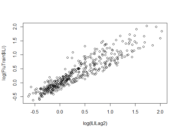
We can see that there is a strong positive relationship between log(ILILag2) and log(ILI).

We can train a linear regression model on the FluTrain dataset to predict the log of the ILI variable using the Queries variable as well as the log of the ILILag2 variable. We can call this model FluTrend2.

FluTrend2 = lm(log(ILI)~Queries+log(ILILag2), data=FluTrain)
summary(FluTrend2)

As can be seen, all three coefficients are highly significant, and the R^2 value is 0.9063.

Moving from FluTrend1 to FluTrend2, in-sample R^2 improved from 0.709 to 0.9063, and the new variable is highly significant. As a result, there is no sign of overfitting, and FluTrend2 is superior to FluTrend1 on the training set.

Evaluating the Time Series Model in the Test Set

So far, we have only added the ILILag2 variable to the FluTrain data frame. To make predictions with our FluTrend2 model, we will also need to add ILILag2 to the FluTest data frame (note that adding variables before splitting into a training and testing set can prevent this duplication of effort).

We can add the new variable with:

ILILag2 = lag(zoo(FluTest$ILI), -2, na.pad=TRUE)
FluTest$ILILag2 = coredata(ILILag2)

From summary(FluTest$ILILag2), we can see that we're missing two values of the new variable.

In this problem, the training and testing sets are split sequentially -- the training set contains all observations from 2004-2011 and the testing set contains all observations from 2012. There is no time gap between the two datasets, meaning the first observation in FluTest was recorded one week after the last observation in FluTrain. From this, we can identify how to fill in the missing values for the ILILag2 variable in FluTest.

The time two weeks before the first week of 2012 is the second-to-last week of 2011. This corresponds to the second-to-last observation in FluTrain. The time two weeks before the second week of 2012 is the last week of 2011. This corresponds to the last observation in FluTrain.

From nrow(FluTrain), we see that there are 417 observations in the training set. Therefore, we need to run the following two commands:

FluTest$ILILag2[1] = FluTrain$ILI[416]
FluTest$ILILag2[2] = FluTrain$ILI[417]

We can obtain the test-set predictions with:

PredTest2 = exp(predict(FluTrend2, newdata=FluTest))

And then we can compute the RMSE with the following commands:

SSE = sum((PredTest2-FluTest$ILI)^2)
RMSE = sqrt(SSE / nrow(FluTest))

Alternatively, you could use the following command to compute the RMSE:

sqrt(mean((PredTest2-FluTest$ILI)^2)).

The test-set RMSE of FluTrend2 is 0.294.

The test-set RMSE of FluTrend2 is 0.294, as opposed to the 0.749 value obtained by the FluTrend1 model.