In August 2006 three researchers (Alan Gerber and Donald Green of Yale University, and Christopher Larimer of the University of Northern Iowa) carried out a large scale field experiment in Michigan, USA to test the hypothesis that one of the reasons people vote is social, or extrinsic, pressure. To quote the first paragraph of their 2008 research paper:

"Among the most striking features of a democratic political system is the participation of millions of voters in elections. Why do large numbers of people vote, despite the fact that ... "the casting of a single vote is of no significance where there is a multitude of electors"? One hypothesis is adherence to social norms. Voting is widely regarded as a citizen duty, and citizens worry that others will think less of them if they fail to participate in elections. Voters' sense of civic duty has long been a leading explanation of vote turnout..."

We will use both logistic regression and classification trees to analyze the data they collected.

The researchers grouped about 344,000 voters into different groups randomly - about 191,000 voters were a "control" group, and the rest were categorized into one of four "treatment" groups. These five groups correspond to five binary variables in the dataset.

• "Civic Duty" (variable civicduty) group members were sent a letter that simply said "DO YOUR CIVIC DUTY - VOTE!"
• "Hawthorne Effect" (variable hawthorne) group members were sent a letter that had the "Civic Duty" message plus the additional message "YOU ARE BEING STUDIED" and they were informed that their voting behavior would be examined by means of public records.
• "Self" (variable self) group members received the "Civic Duty" message as well as the recent voting record of everyone in that household and a message stating that another message would be sent after the election with updated records.
• "Neighbors" (variable neighbors) group members were given the same message as that for the "Self" group, except the message not only had the household voting records but also that of neighbors - maximizing social pressure.
• "Control" (variable control) group members were not sent anything, and represented the typical voting situation.
• Additional variables include sex (0 for male, 1 for female), yob (year of birth), and the dependent variable voting (1 if they voted, 0 otherwise).

We can load the dataset gerber.csv into R by using the read.csv command:

gerber = read.csv("gerber.csv")

Then we can compute the percentage of people who voted by using the table function:

table(gerber$voting)

The output tells us that 235,388 people did not vote, and 108,696 people did vote. This means that 108696/(108696+235388) = 0.316 of all people voted in the election.

In order to know which of the four "treatment groups" had the largest percentage of people who actually voted (voting = 1), we can type the following code in R.

tapply(gerber$voting, gerber$civicduty, mean)
tapply(gerber$voting, gerber$hawthorne, mean)
tapply(gerber$voting, gerber$self, mean)
tapply(gerber$voting, gerber$neighbors, mean)

The variable with the largest value in the "1" column has the largest fraction of people voting in their group - this is the Neighbors group.

We can build the logistic regression model with the following command:

LogModel = glm(voting ~ civicduty + hawthorne + self + neighbors, data=gerber, family="binomial")

If we look at the output of summary(LogModel), we can see that all of the variables are significant.

In order to calculate the accuracy of Logistic regression model with a threshold of greater then 0.3:

predictLog = predict(LogModel, type="response")
table(gerber$voting, predictLog > 0.3)

We can compute the accuracy of the sum of the true positives and true negatives, divided by the sum of all numbers in the table:

(134513+51966)/(134513+100875+56730+51966) = **0.542**

For a threshold of 0.5

table(gerber$voting, predictLog > 0.5)

We can compute the accuracy of the sum of the true positives and true negatives, divided by the sum of all numbers in the table:

(235388+0)/(235388+108696) = **0.684**

We can compute the AUC with the following commands (if your model's predictions are called "predictLog"):

library(ROCR)
ROCRpred = prediction(predictLog, gerber$voting)
as.numeric(performance(ROCRpred, "auc")@y.values)

Even though all of our variables are significant, our model does not improve over the baseline model of just predicting that someone will not vote, and the AUC = 0.5308461 is low. So while the treatment groups do make a difference, this is a weak predictive model.

Trees

We will now try out trees. We will build a CART tree for voting using all data and the same four treatment variables we used before. We don't set the option method="class" - we are actually going to create a regression tree here. We are interested in building a tree to explore the fraction of people who vote, or the probability of voting. We’d like CART to split our groups if they have different probabilities of voting. If we used method=‘class’, CART would only split if one of the groups had a probability of voting above 50% and the other had a probability of voting less than 50% (since the predicted outcomes would be different). However, with regression trees, CART will split even if both groups have probability less than 50%.

CARTmodel = rpart(voting ~ civicduty + hawthorne + self + neighbors, data=gerber)

If we plot the tree, with prp(CARTmodel), we should just see one leaf! There are no splits in the tree, because none of the variables make a big enough effect to be split on.

Now let's build the tree using the command:

CARTmodel2 = rpart(voting ~ civicduty + hawthorne + self + neighbors, data=gerber, cp=0.0)

to force the complete tree to be built. Then plot the tree. What do you observe about the order of the splits?

We can plot the tree with prp(CARTmodel2).

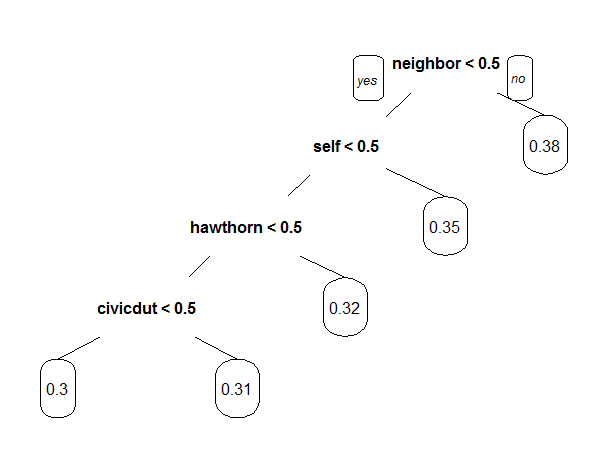
As, we saw initially that the highest fraction of voters was in the Neighbors group, followed by the Self group, followed by the Hawthorne group, and lastly the Civic Duty group. And we see here that the tree detects this trend.

Using only the CART tree plot, we can determine what fraction (a number between 0 and 1) of "Civic Duty" people voted which is the value at the bottom right leaf 0.31

Let's make a new tree that includes the "sex" variable, again with cp = 0.0. Notice that sex appears as a split that is of secondary importance to the treatment group.

CARTmodel3 = rpart(voting ~ sex +civicduty + hawthorne + self + neighbors, data=gerber, cp=0.0)
prp(CARTmodel3)

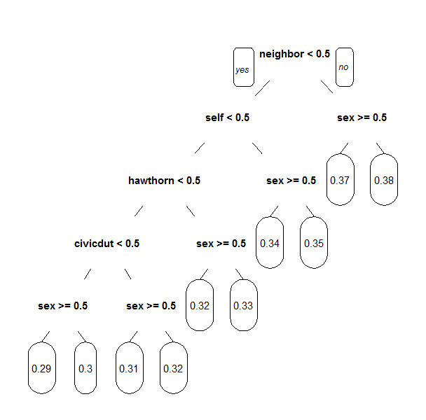
We can see that there is a split on the "sex" variable after every treatment variable split. For the control group, which corresponds to the bottom left, sex = 0 (male) corresponds to a higher voting percentage.

For the civic duty group, which corresponds to the bottom right, sex = 0 (male) corresponds to a higher voting percentage.

Interaction Terms

We know trees can handle "nonlinear" relationships, e.g. "in the 'Civic Duty' group and female", but it is possible to do the same for logistic regression. First, let's explore what trees can tell us some more.

Let's just focus on the "Control" treatment group. Let's Create a regression tree using just the "control" variable, then create another tree with the "control" and "sex" variables, both with cp=0.0.

CARTcontrol = rpart(voting ~ control, data=gerber, cp=0.0)
CARTsex = rpart(voting ~ control + sex, data=gerber, cp=0.0)

Then, plot the "control" tree with the following command:

prp(CARTcontrol, digits=6)

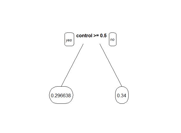
The split says that if control = 1, predict 0.296638, and if control = 0, predict 0.34. The absolute difference between these is 0.043362.

prp(CARTsex, digits=6)

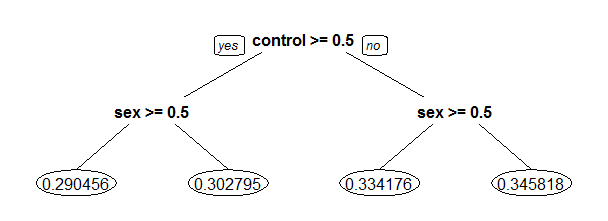
The first split says that if control = 1, go left. Then, if sex = 1 (female) predict 0.290456, and if sex = 0 (male) predict 0.302795. On the other side of the tree, where control = 0, if sex = 1 (female) predict 0.334176, and if sex = 0 (male) predict 0.345818. So for women, not being in the control group increases the fraction voting by 0.04372. For men, not being in the control group increases the fraction voting by 0.04302. So men and women are affected about the same by NOT being in the control group (being in any of the four treatment groups).

Going back to logistic regression now,Let's create a model using "sex" and "control".

LogModelSex = glm(voting ~ control + sex, data=gerber, family="binomial")

If we look at the summary of the model, we can see that the coefficient for the "sex" variable is -0.055791. This means that women are less likely to vote, since women have a larger value in the sex variable, and a negative coefficient means that larger values are predictive of 0.

The regression tree calculated the percentage voting exactly for every one of the four possibilities (Man, Not Control), (Man, Control), (Woman, Not Control), (Woman, Control). Logistic regression has attempted to do the same, although it wasn't able to do as well because it can't consider exactly the joint possibility of being a women and in the control group.

We can quantify this precisely. Let's create the following dataframe (this contains all of the possible values of sex and control), and evaluate our logistic regression using the predict function (where "LogModelSex" is the name of your logistic regression model that uses both control and sex):

Possibilities = data.frame(sex=c(0,0,1,1),control=c(0,1,0,1))
predict(LogModelSex, newdata=Possibilities, type="response")

The four values in the results correspond to the four possibilities in the order they are stated above ( (Man, Not Control), (Man, Control), (Woman, Not Control), (Woman, Control) ). the absolute difference between the tree and the logistic regression for the (Woman, Control) case is:

The CART tree predicts 0.290456 for the (Woman, Control) case, and the logistic regression model predicts 0.2908065. So the absolute difference, to five decimal places, is 0.00035.

So the difference is not too big for this dataset, but it is there. We're going to add a new term to our logistic regression now, that is the combination of the "sex" and "control" variables - so if this new variable is 1, that means the person is a woman AND in the control group. We can do that with the following command:

LogModel2 = glm(voting ~ sex + control + sex:control, data=gerber, family="binomial")

This coefficient is negative, so that means that a value of 1 in this variable decreases the chance of voting. This variable will have VALUE 1 if the person is a woman and in the control group.

Running the same code as before to calculate the average for each group:

predict(LogModel2, newdata=Possibilities, type="response")

The logistic regression model now predicts 0.2904558 for the (Woman, Control) case, so there is now a very small difference (practically zero) between CART and logistic regression.

This example has shown that trees can capture nonlinear relationships that logistic regression can not, but that we can get around this sometimes by using variables that are the combination of two variables.

But, We should not use all possible interaction terms in a logistic regression model due to overfitting. Even in this simple problem, we have four treatment groups and two values for sex. If we have an interaction term for every treatment variable with sex, we will double the number of variables. In smaller data sets, this could quickly lead to overfitting.